Interactive Medical Simulation Toolkit (iMSTK)

User Documentation

Introduction

iMSTK is a free and open source software toolkit written in C++ that aids rapid prototyping of interactive multi-modal surgical simulations. It provides a highly modular and easy to use framework that can be extended and be interfaced with other third-party libraries for the development of medical simulators without restrictive licenses.

iMSTK supports all major platforms (MacOS, Linux, Windows) with the ability to build all the dependencies automatically using CMake. Current features include (a) support for a Vulkan and a VTK rendering backend, (b) VR support, (c) External tracking device hardware support, (d) linear and nonlinear FEM and PBD (including fluids), (e) standard numerical solvers such as Newton, CG, Gauss-Seidel, and (e) continuous collision detection.

This documentation is designed to provide an overview of iMSTK, introductory concepts needed to comprehend the framework, its component modules and how they interact to help build simulations. For implementational level details of the modules and their classes, please refer to the code. The chapters that follow will describe details of how to build iMSTK, elements of the simulation scenario and how these elements are connected using iMSTK modular architecture followed by detailed description of each of the major modules. The final chapter includes a walk-through of the code of an all-inclusive example to help the readers to quickly build their application.

Setup for Development

iMSTK and its external dependencies can be configured and built from scratch Cmake to create a super-build on UNIX (MAC, Linux) and Windows platforms. The instructions below describe this process in detail.

Configuration and Build

CMake should be used to configure the project on every platform. Please refer to CMake’s official page to read about how to configure using CMake.

Linux/MacOSx

Type the following commands from the same location you cloned the

>> mkdir iMSTK_build
>> cd iMSTK_build
>> cmake ../iMSTK    # path to source directory
>> make -j4 #to build using *4* cores

This will configure the build in a directory adjacent to the source directory. To easily change some configuration variables such as CMAKE_BUILD_TYPE, use ccmake instead of cmake.

One can also use Ninja for a faster build instead of Unix Makefiles. To do so, configure the cmake project with -GNinja

>> cmake -GNinja
>> ../iMSTK
>> ninja

This will checkout, build and link all iMSTK dependencies. When making changes to iMSTK base source code, you can then build from the Innerbuild directory.

Windows

Run CMake-GUI and follow the directions described on CMake’s official page. You need to choose which version of Visual Studio that you would like to use when configuring the project. Make sure to select Microsoft Visual Studio C++ 12 2015 or later. CMake will generate a iMSTK.sln solution file for Visual Studio at the top level. Open this file and issue build on all targets, which will checkout, build and link all iMSTK dependencies. When making changes to iMSTK base source code, you can then build from the iMSTK.sln solution file located in the Innerbuild directory.

Running Examples

The default CMake configuration builds the examples as part of the inner build. The executables including other targets required to run the executables are placed in the <imstk build dir>/install/bin directory. The execurables can either be run through command line or double clicking.

Options at Configure Time

Phantom Omni Support

To support the Geomagic Touch (formerly Sensable Phantom Omni) haptic device, follow the steps below:

1. Install the OpenHaptics SDK as well as the device drivers:
   1. for Windows
   2. for Linux
2. Reboot your system.
3. Configure your CMake project with the variable iMSTK_USE_OpenHaptics set to ON.
4. After configuration, the CMake variable OPENHAPTICS_ROOT_DIR should be set to the OpenHaptics path on your system.

Vulkan Rendering Backend

To use the Vulkan renderer instead of the default VTK, follow these steps:

1. Download the VulkanSDK
2. Download your GPU vendor’s latest drivers.
3. Enable the iMSTK_USE_Vulkan option in CMake.

Note

The examples that depend on this option being on at configure time will not build automatically if this option is not selected.

Building Examples

The examples that demonstrate the features and the usage of iMSTK API can be optionally build. Set BUILD_EXAMPLES to ON the examples needs to be built.

Virtual Reality Support

iMSTK can optionally display the render frames to the HMD instead of the default 2D screen. In order to enable VR via openVR, set iMSTK_ENABLE_VR to ON.

Audio Support

iMSTK has the ability to play audio streams at runtime. In order to enable Audio, set iMSTK_ENABLE_AUDIO to ON.

Uncrustify Support

iMSTK follows specific code formatting rules. This is enforced through Uncrustify. For convenience, iMSTK provides the option to build uncrustify as a target. To enable this set iMSTK_USE_UNCRUSTIFY to ON.

Multithreaded build

The build will be configured to be multithreaded with 8 threads. This can be changed by modifying the iMSTK_NUM_BUILD_PROCESSES to a positive intiger.

External Dependencies

iMSTK builds upon well-established open-source libraries. Below is the list of iMSTK’s external dependencies and what they are used for in IMSTK.

Library	Usage
Eigen	linear algebra (vectors, matrices, basic matrix algebra etc.)
VRPN	Interfacing with external hardware devices.
SFML	Audio support
G3log	Asynchronous logging
Google Test	Unit testing
OpenVR	HMD-based Virtual reality support
SCCD	Continuous collision detection
Uncrustify	Enforcing code formatting
VEGA Fem	Rendering, visualization and filters
VTK	Finite element support
TBB	Intel Thread building block for multithreading
Assimp	Import/export standard 3D mesh formats
PhysX	Rigid body dynamics

Secondary external dependencies include glfw, gli, glm, LibNiFalcon, Linusb, and PThread.

Overview of iMSTK

Elements of a Scene

In iMSTK, a collection of ‘scene objects’, their interaction graph and inanimate entities like (lights, camera etc.) form a scene. Scene objects are defined with internal states (eg: displacements, temperature) that may be governed by a mathematical law. The interaction between the scene objects is specified by a collision detection and collision handling. The interaction laws are encoded in the collision handling.

Module

A iMSTK module facilitates execution of a set callback function in a separate thread. Any simulation related logic is executed via one module or the another. For example, the devices often require a separate thread for I/O which will be facilitated through the imstkModule class. At any given instance in time, a module can be in one of the following states:

1. STARTING
2. RUNNING
3. PAUSING
4. PAUSED
5. TERMINATING
6. INACTIVE

the module also allows specifying custom function callbacks that will be called at the start or end of the execution frame. The examples demonstrate the usage of these callbacks.

Simulation Manager

The simulation manager is a high-level class that drives the entire simulation. Some of the functionalities of the simulation manager include:

1. Addition and removal of a scene
2. Execution control of a currently active scene: Start, Run, Pause, Reset, End
3. Setting active scene
4. Adding and remove modules (run in separate threads)
5. Starting the renderer

The simulation manager initialized in the following modes:

• rendering: Launch the simulation with a render window
• runInBackground: Launch the simulation without a render window but keeps looping the simulation
• backend: Launch the simulation without a render window and returns the control

These modes are enumerated at imstk::SimulationManager::Mode. The default mode is rendering. The usage is as follows.

auto simManager   = std::make_shared<SimulationManager>(
                          SimulationManager::Mode::rendering /* rendering mode*/,
                          false /*no VR mode*/);

Scene Manager

The scene manager is a module (which runs in a different thread) that executes each frame of the simulation in the scene on-demand. Each frame is triggered by the simulation manager. The simulation workflow described below is implemented in the runModule() function of the sceneManager.

Scene Objects

The scene object encapsulates an individual actor that has an internal state which is governed by a mathematical formulation (force model described later). The internal state (eg: deformation field, temperature) exists over a finite geometry; therefore each scene object contains geometric representations for visual, collision and the physics modules to utilize. The geometric representations could be the same or separate (for example one might want to do collisions on coarser geometric representations while the physics is resolved on a denser representation) for these three modules. The geometric representation can be a collection of points with or without connectivity or even a standard shape.

Geometry Mappers

The consistency between the visual, collision and the physics geometric representations is maintained using geometry mappers. At any given simulation frame, all the internal states are updated, collisions are computed, interactions are resolved and the new states are passed via mappers to the renderer to update the visuals. iMSTK provides standard mappers to map for example, displacement from volumetric mesh the displayed mesh which is a surface. Arbitrary custom mappers can be defined by the user.

Collision Graph

The interaction graph describes the interaction between the scene objects. Below is a sample code to describe the interaction between an elastic body and a rigid sphere using penalty-based collision response and PointSetToSphere collision detection.

// Create a collision graph
auto graph = scene->getCollisionGraph();
auto pair = graph->addInteractionPair(elastibBody,
                                    Sphere,
                                    CollisionDetection::Type::PointSetToSphere,
                                    CollisionHandling::Type::Penalty,
                                    CollisionHandling::Type::None);

Note

In cases where both the objects are deformable, collision response can be prescribed both ways. More details on the collision detection and response can be found in their respective sections later.

Inanimate Scene Elements

Background elements of the scene that are not necessarily visible or affect the simulation are the lights and camera. They are described in detail in the rendering section.

Simulation Workflow

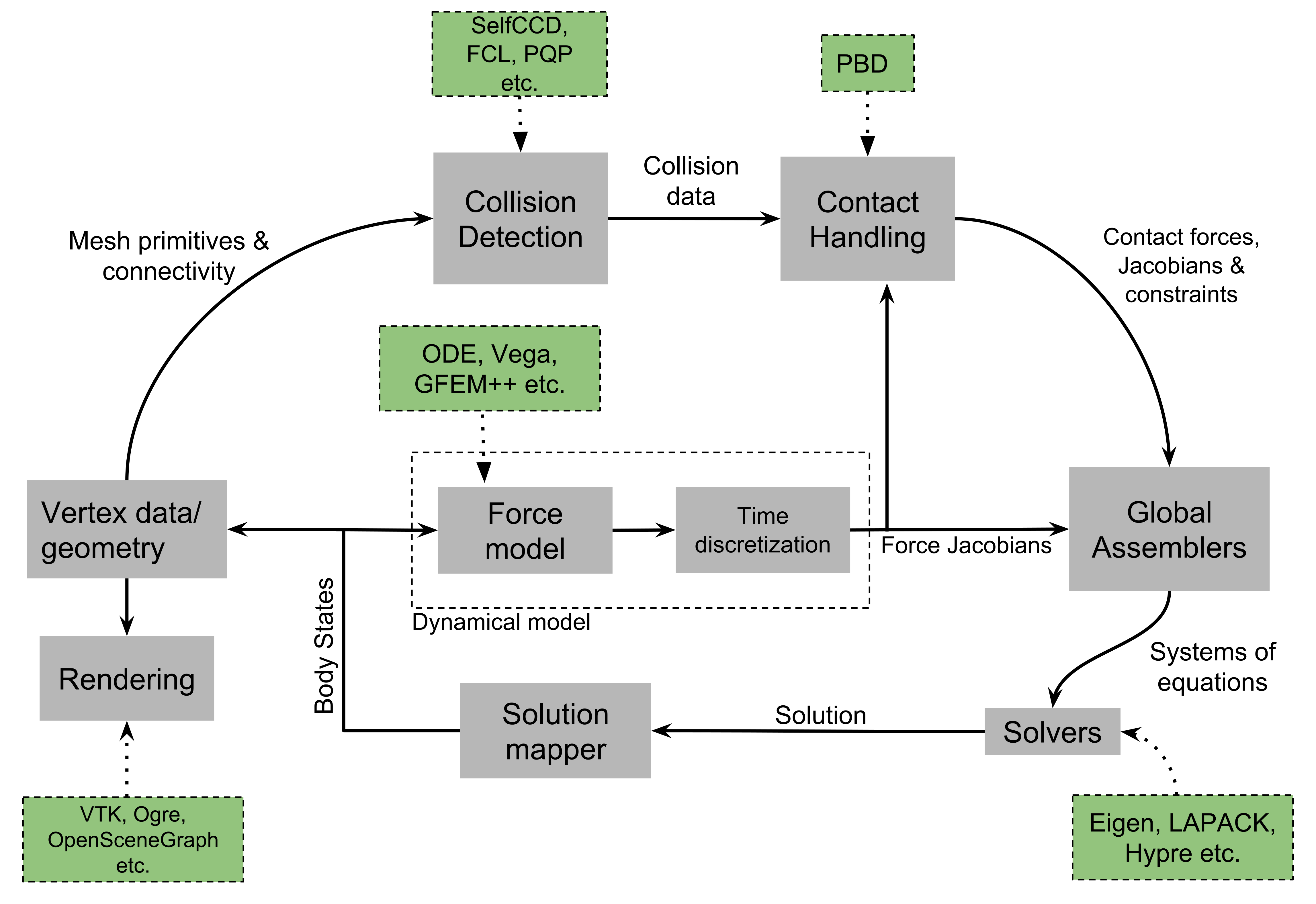
The flowchart above shows the brief overview of the simulation workflow. At any given frame the force vectors and the Jacobian matrices are computed and passed on to the assembly. The collision detection computes the intersecting scene objects based on the latest configuration available from and the collision data is passed to the contact handling module. Depending on the type of contact handler either the forces or constraints based are passed to the assembler. The assembled assembles the discrete set of equations that will be solved by the solver chosen. Once the solution is obtained the geometry mappers deconstruct this and update the visual geometries. The mappers further update the physics and collision mesh representations (if they happen to be different). This is continued until the user terminates or pauses the simulation.

Object Geometry

iMSTK handles a wide variety of geometric types that will be used for visual representations of the scene objects, collision computations or as input domain for physics formulations. The geometry is broadly classified as (a) Analytic (parameterized) and (b) Discrete geometry.

Analytical Geometry

Analytic geometry represents standard shapes that can be fully specified few parameters. iMSTK supports the following 3D shapes.

• Sphere: Specified by radius and center
• Cube: Specified by length of the side and the center
• Plane: Specified by normal and any point on a plane
• Capsule: Specified by radius, length (between the centers of end planes of the cylindrical section) and position (of the center of the cylinder)
• Cylinder: Specified by the radius, length and the position (of the center of the cylinder)

The default position is (0,0,0) and the defaulted to unit length along the cylinder axis. For rendering purposes, the internal representation of the above shapes is mapped to the VTK data structures.

Discrete Geometry

Discrete geometry is where a shape is represented by a collection of primitives such as points, triangles, tetrahedron, hexahedron etc. iMSTK currently supports, point clouds, surface mesh, and unstructured volumetric meshes composed of tetrahedral primitives.

Surface Mesh

Surface meshes consist of vertices and triangles. The vertices contain information such as position, normals, UV coordinates, and tangents. Each triangle contains the index of the three vertices. Surface mesh normals consider UV seams so that when deformation occurs, the normals look smooth even when the vertices are duplicated.

Volumetric Mesh

The volumetric mesh is composed of vertices and tetrahedral elements. The vertices can also hold additional scalar data for visualization purposes.

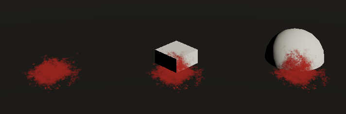
Decals (Vulkan only)

This geometry type actually consists of two related classes: decals and decal pools. A decal a unique object that can project onto underlying opaque geometry. The projection is along the Z-axis. A decal pool is a collection decals. Memory is preallocated ahead of time on the GPU side to support additional decals.

In terms of how the decals are rendered, decals are instanced and share the same material. Therefore, materials should only be assigned to the decal pool, rather than the decal. This makes a decal pool a relatively heavy object while decals are lightweight. Decals blend to the layer underneath, inheriting their normals, meaning that normal maps will not work. Unlike opaque geometry, decals are only rendered once and cannot cast shadows.

Decals have a projection box that is by default one meter in each direction. This can be scaled by setting the scale of each decal. Opaque geometry that intersects this box will have the decal’s material projected onto it. If the decal is parallel to a surface, then the projection will look severely stretched. To avoid this, rotate the decal by a small amount. If the decal is facing the wrong direction, then it will be invisible.

Rendering

iMSTK rendering is powered by two rendering APIs: VTK (default) and Vulkan.

VTK Backend

The VTK backend is provided to allow for advanced visualization features for debugging and visualization application behavior such as physics.

Vulkan Backend

The Vulkan backend concentrates on photorealistic graphics and uses more much aggressive/expensive approaches to achieve this goal. Currently, the Vulkan backend follows concepts from physically-based rendering (PBR). This doesn’t have a clear definition, but the route taken by the Vulkan backend consists of:

• Linear color space
• Microfacet specular BRDF with energy conservation
• High dynamic range with filmic tonemapping
• Post processing that operates based on more physical values

Render Material System

A render material holds information on the appearance of an item. This information includes:

• Textures
• Display modes (such as wireframe)
• Values (such as roughness)
• Shader details

Although a material is a higher level abstraction, it has a large impact on performance.

The materials properties that are available in iMSTK are described below along with their definitions:

Property	Definition
Roughness	VTK: influences how smooth a surface is for Blinn-Phong. This doesn’t have a precise physical meaning. Vulkan: influences roughness. This value is actually squared to allow for more precision for lower roughness values. This has a precise physical meaning.
Metalness	VTK: influences specular color. Vulkan: has a physical meaning, influencing both the specular color and Fresnel strength.
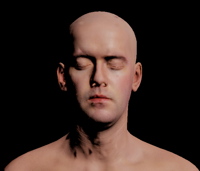
SSS	Vulkan: influences the radius and strength of the subsurface scattering post-processing pass.
Tessellation	Vulkan: currently tessellates the mesh

Texture Manager

The texture manager caches textures already in use. Generally most of the GPU memory in use by the application will be consumed by textures, so it’s important to avoid redundantly uploading textures. The texture manager currently uses multiple parameters to detect redundancy including file path and texture type. It’s possible for the same image file to be loaded more than once if it’s used in different ways (e.g., using the same image for roughness and albedo). This is by design because different types of texture can be optimized in different image formats to save space.

Lights

Note

The intensity of the light can exceed 1.0, which gets clamped in the VTK backend but is smoothed in the Vulkan backend due to the tonemapping. Thus, the resulting appearance will be different.

Directional Lights

Directional lights have a direction, an intensity, and a color. In the Vulkan renderer, they can also cast shadows.

Point Lights

Point lights have a position, an intensity, and a color. Light rays are calculated coming out from the center of the point light.

Spot Lights

Spot lights are a special case of point lights that also have an angle cut off along a certain direction.

Image-Based Lighting (Vulkan only)

Image-based lighting (IBL) allows the scene to be illuminated by a surrounding light source. This can be used in the Vulkan backend. To use it, a global IBL probe object must be created and assigned to the scene. The object takes three textures: an irradiance cubemap, a radiance cubemap, and a BRDF lookup table. The two cubemap textures must be in DDS format, and should also use high-dynamic range for the best results. The radiance cubemap in particular should be mipmapped.

Debug Rendering

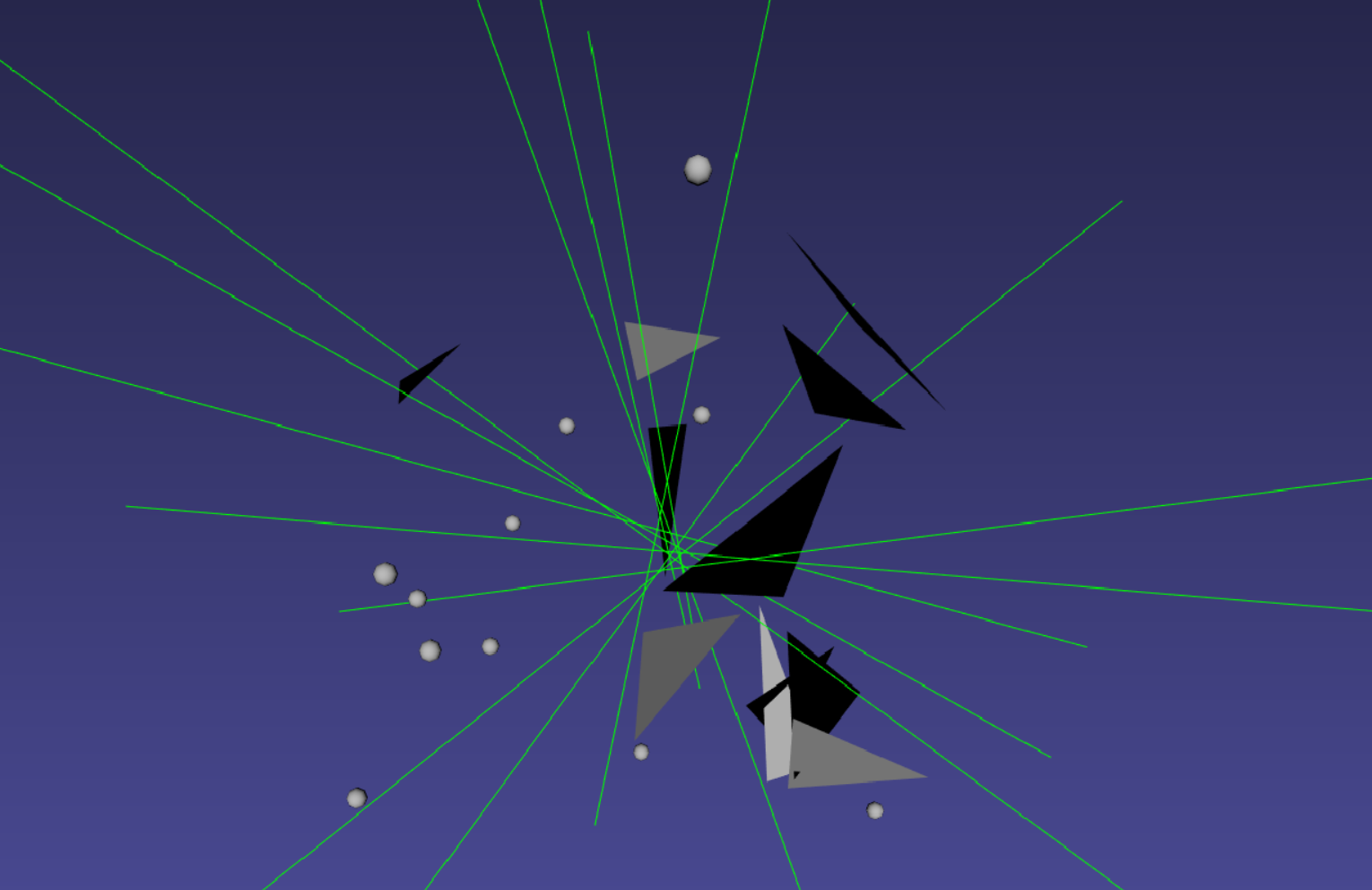
Developers often need to visualize geometrical primitives that are not necessarily part of the scene object geometry. For example, octree grid which is not part of the scene objects need to be optionally displayed in order to monitor accuracy. DebugRenderGeometry class is designed for this purpose. Users can add arbitrirary number of points, lines and traingle primitives at runtime to the scene that will be rendered along with the regular scene geometry. One difference to be noted is that each geometric primitives should be by themselves meaning they are not connected to each other even though in reality they may be. While in some cases this is redundant but offers greater flexibility due to greatly reduced bookkeeping of the connectivity. The screenshot below shows randomly created primitives of the debug geometry displayed in the scene.

Usage:

// Create lines for debug rendering
auto debugLines = std::make_shared<DebugRenderLines>("Debug Lines");
auto material   = std::make_shared<RenderMaterial>();
material->setBackFaceCulling(false);
material->setDebugColor(Color::Green);
material->setLineWidth(2.0);
debugLines->setRenderMaterial(material);
scene->addDebugGeometry(debugLines);

...

// At runtime add points that represent lines
debugLines->appendVertex(p);
debugLines->appendVertex(q);

Custom On-screen text

Often times it is useful to display additional information on the render window. iMSTK’s VTKTextStatusManager class makes this possible. Below is the snippet from the DebugRendering example that displays the number of debug primitives currently dislpayed in the render window.

auto statusManager = viewer->getTextStatusManager();
statusManager->setStatusFontSize(VTKTextStatusManager::Custom, 30);
statusManager->setStatusFontColor(VTKTextStatusManager::Custom, Color::Orange);

statusManager->setCustomStatus("Primatives: " +
                       std::to_string(debugPoints->getNumVertices()) + " (points) | " +
                       std::to_string(debugLines->getNumVertices() / 2) + " (lines) | " +
                       std::to_string(debugTriangles->getNumVertices() / 3) + " (triangles)"
            );

The font size, color, display corner and padding spaces of the texture manager can be configured.

Note

This feature is only available with the VTK rendering backend.

Collision Detection

A typical simulation scenario can feature multiple objects interacting with each other in real-time. Collision detection (CD) is the first step to resolving the physical contact between the objects that are typically represented using a collection of simpler geometric primitives such as vertices, edges, and triangles. Collision detection algorithms are tasked to not only detect and but also report the geometric details of all the points of contact. Accurately and efficiently detecting collisions between interacting objects and handling them using appropriate mechanisms can enhance the accuracy and the realism of application.

Collision detection is typically divided into two phases: (a) the broad phase where a set of candidate collision primitive pairs is identified, and (b) the narrow phase where the geometric intersection tests are performed on these candidate primitive pairs [cd1]. The narrow phase intersection tests are computationally expensive and hence the broad phase algorithms aim to achieve smallest possible candidate set of collision pairs (with all the actual collision pairs being a subset) with a minimal computational cost.

The broad phase algorithms typically employ hierarchical spatial partitioning data structures such as octrees or BVH to organize and store geometric information for efficient retrieval and processing. Collision detection has been researched extensively in the computer graphics area and its implementation can vary widely depending on the assumptions that are valid for the problem at hand and the target hardware.

Broad Phase

iMSTK’s broad phase uses octree data structure to perform quick culling of the primitive collision pairs.

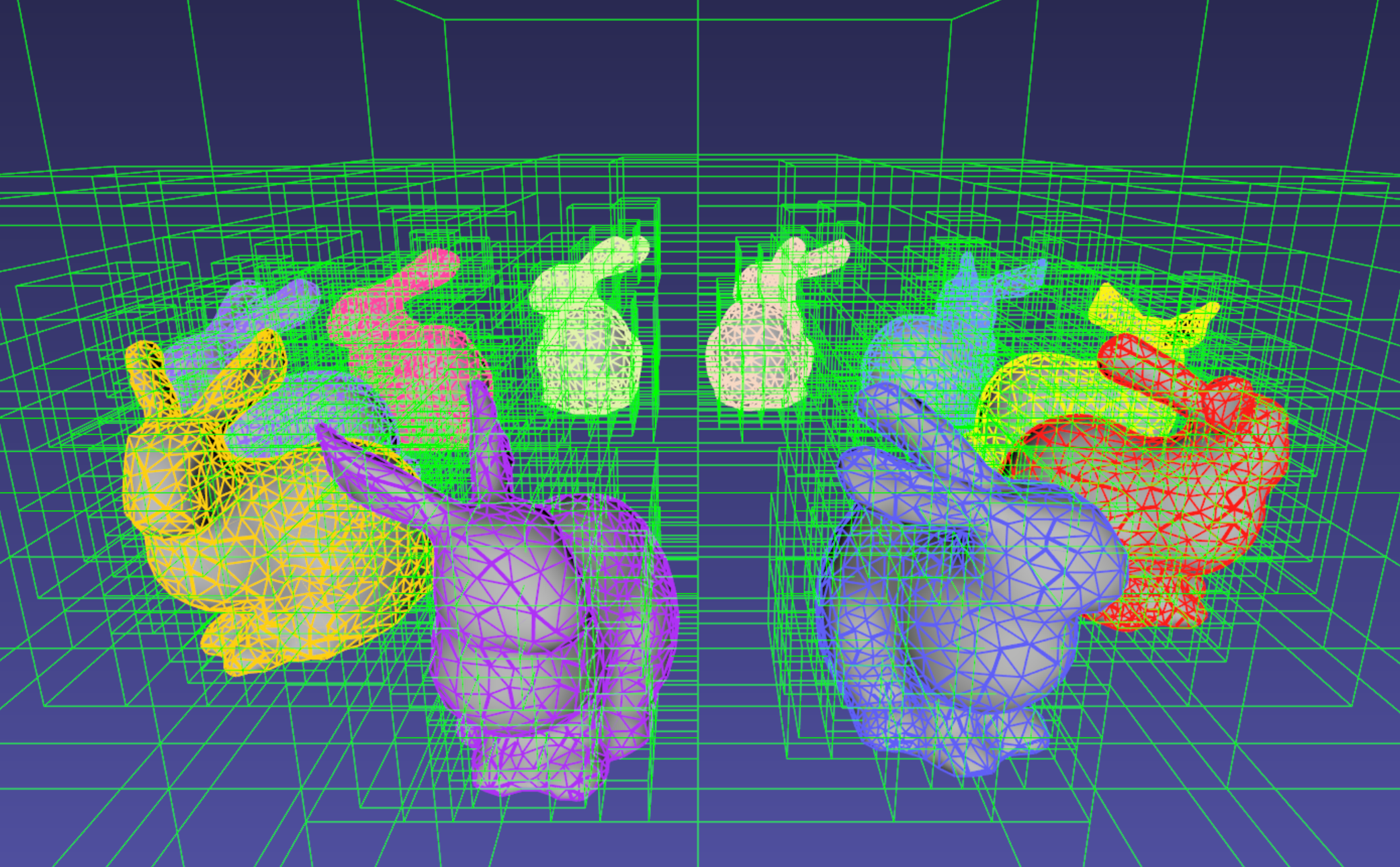
Octree Collision

An octree is an axis-aligned hierarchical data structure that is generated by recursively subdividing the axis-aligned bounding box (AABB) into eight equally-sized cells as necessary. Generally speaking, the choice of whether to subdivide an octree node or not depends on the density of information present at that node which in this case is the geometry of the primitives.

A brute-force way to find collisions between a set of n disjointed primitives can mean testing all the possible pairs which can be computationally prohibitive requiring O(n2) work. The broad phase of the collision detection aims to efficiently eliminate a subset of primitive pairs (also called culling) that are guaranteed not to collide thus leaving only fewer combinations for which expensive geometric tests are performed. An efficient broad phase algorithm aims to minimize the size of the left out pairs while still retaining guarantees (i.e., all the colliding pairs are part of this set).

The broad phase of the octree collision detection consists of two stages:

Tree update: In this step, each primitive under consideration for collision are assigned to an octree node depending on the spatial extent, position, and orientation. For this purpose, the AABB of each primitive is recursively checked against the cells starting at the root node. A primitive will be assigned to a node if either the primitive size exceeds the extent of the cells of the child nodes or the current node cannot be further subdivided due to a preset limit on the maximum depth of the octree.

Culling: This step aims to take advantage of the spatial partitioning of the octree and eliminate as many non-colliding primitive pairs as possible from the list of all the possible pairs. Given a primitive, it is first checked for intersection with the boundary of the root node. If the primitive does not intersect with the node boundary, no further operation is performed with the tree node. Otherwise, it is then tested for intersection with all the primitives stored in the tree node. This process is then recursively called on the child nodes until reaching leaf nodes. With n primitives, detecting a collision between them has a time complexity O(nhk) in the worst case, where h is the height of the octree, and k is the maximum number of primitives at any octree node. In practice, h is around 10 and most primitives are stored at the leaf nodes; thus, the cost of detecting collision for each primitive is bounded and can be very cheap.

In iMSTK, OctreeBasedCD class embeds the implementation of the above-described functionality. Users can both access the list of primitives at any given node in the hierarchy and collision data through public API. The code snippet below shows how an octree is built and used to detect collision between two mesh objects that contain triangle primitives:

// Initialize the octree
OctreeBasedCD octreeCD(Vec3d(0, 0, 0), // Center of the root node
                       100.0, // Side length of the root node
                       0.1);  // Minimum allowed width for any octree cell

// Add mesh objects containing triangle primitives to the octree
octreeCD.addTriangleMesh(triMesh_1);
octreeCD.addTriangleMesh(triMesh_2);

// Build the Octree
octreeCD.build();

// Add collision pairs between meshes
octreeCD.addCollisionPair(triMesh_1, triMesh_2,
                        CollisionDetection::Type::SurfaceMeshToSurfaceMesh);

At any given frame during the simulation, querying the generated collision data:

// Update octree (primitives might have moved in the prior frame)
octreeCD.update();

// Access the collision data for the mesh pair
const auto& colData = octreeCD.getCollisionPairData(
                           indx1,  // Global index of triMesh_1
                           indx2); // Global index of triMesh_2

Narrow Phase

iMSTK provides numerous narrow phase intersection tests between primitives and are implemented as static functions within the imstk::NarrowPhaseCD namespace. The current list of functions provide the following intersection tests:

• BidirectionalPlane-Sphere
• UnidirectionalPlane-Sphere
• Sphere-Cylinder
• Sphere-Sphere
• Point-Capsule
• Point-Plane
• Point-Sphere
• Triangle-Triangle
• Point-Triangle

Continuous collision detection

Continuous collision detection (CCD) algorithm extends the collision in time thereby capturing the collisions otherwise missed by the traditional collision detection algorithms. CCD is typically used in cases where there are fast moving objects in the scene causing the traditional discrete CD fail to detect collisions. CCD performs collision of the volumes swept by the colliding primitives in order to detect the exact time of intersection (if any). In iMSTK, CCD is made available through selfCCD library. The class SurfaceMeshToSurfaceMeshCCD imlpements this feature. Note that in addition to the geometry information resulting from intersection tests, CCD outputs a scalar ‘time’ that is normalized between 0-1 for the time period between the frames being considered.

Collision data

The collision data that is produced as a result of the collisions and is passed on to the collision handling module for processing. Any collision detection algorithm results in one or more of the following data types:

• Vertex-Triangle
• Edge-Edge
• Mesh-AnalyticalGeometry
• Point-Tetrahedron
• Position-Direction

The definitions of the above collifion data types can be found in imstkCollisionData.h.

Collision Handling

Collision handling determines what needs to be done in the event of collision. The collision data obtained from the CD module is used to either compute the response forces or generate constraints that will be solved along with the internal forces. iMSTK currently supports penalty, linear projection constraints, PBD collision constraints, virtual coupling and picking collision handling.

Physics

iMSTK is designed to accommodate varied physics-based formulations that govern the internal states ascribed to the scene objects. The architecture is designed in such a way that different physical modalities such as 3D elastic objects, fluids (such as liquids and smoke), thin elastic sheets, elastic strings can be accommodated with the choice of different formulations for each modality.

Modality	Formulation	Usage
3D Elastic object	FE SPH Meshless	Tissue Generic elastic solids
Fluids	Finite Volume SPH PBD	Blood Smoke
Elastic objects in 3D with 2D topology	PBD FE	Thin tissue layers Cloth-like objects in skill trainers
Elastic objects 3D with 1D topology	PBD FE	Suture thread
Other: Heat diffusion, electric potential	FE	Use of energy in surgery

The table above lists various modalities, ]physics based formulations that help realized them and their potential usage in medical simulations. While the architecture itself allows extension to most modalities and their formulations, only a subset of them are currently available in iMSTK.

In iMSTK, the partial differential equations that describes the evolution of the physical quantities both in space and time are modeled using dynamicalModel class. The dynamical model is composed of the internal force model and the time stepping scheme which are designed to take in the current internal states and produce force (analogous) vector and Jacobian matrices to be used by the solvers.

3D Deformable Objects

iMSTK supports elastic solids both using finite element (FE) and PBD. FE support is only limited to tetrahedral elements while the PBD formulation is agnostic to the underlying mesh.

auto dynaModel = std::make_shared<FEMDeformableBodyModel>();
dynaModel->configure(iMSTK_DATA_ROOT"/asianDragon/asianDragon.config");
dynaModel->setTimeStepSizeType(TimeSteppingType::realTime);
dynaModel->setModelGeometry(volTetMesh);

// Create and add Backward Euler time integrator
auto timeIntegrator = std::make_shared<BackwardEuler>(0.001);

dynaModel->setTimeIntegrator(timeIntegrator);

FE dynamical model can be configured by using an external configuration file. The configuration file specifies (a) an external file listing the IDs of the nodes that are fixed, (b) density, (c) Damping coefficients, (d) elastic modulus, (e) Poisson’s ratio, (f) the choice of FE formulation available. The formulation that are available are (i) Linear (ii) Co-rotation (iii) invertable (iv) Saint-Venant Kirchhoff. Currently backward Euler is the only time stepping that is available in iMSTK.

Below is a sample code that shows the configuration of an elastic object with PBD formulation.

auto deformableObj = std::make_shared<PbdObject>("Beam");
auto pbdModel = std::make_shared<PbdModel>();
pbdModel->setModelGeometry(volTetMesh);
pbdModel->configure(/*Number of Constraints*/ 1,
                    /*Constraint configuration*/ "FEM StVk 100.0 0.3",
                    /*Mass*/ 1.0,
                    /*Gravity*/ "0 -9.8 0",
                    /*TimeStep*/ 0.01,
                    /*FixedPoint*/ "51 127 178",
                    /*NumberOfIterationInConstraintSolver*/ 5);

Note that unlike FE, for the case of PBD formulation, the choice of time stepping scheme and solver is restricted in choice resulting in a compact API to prescribe the entirety of the object configuration.

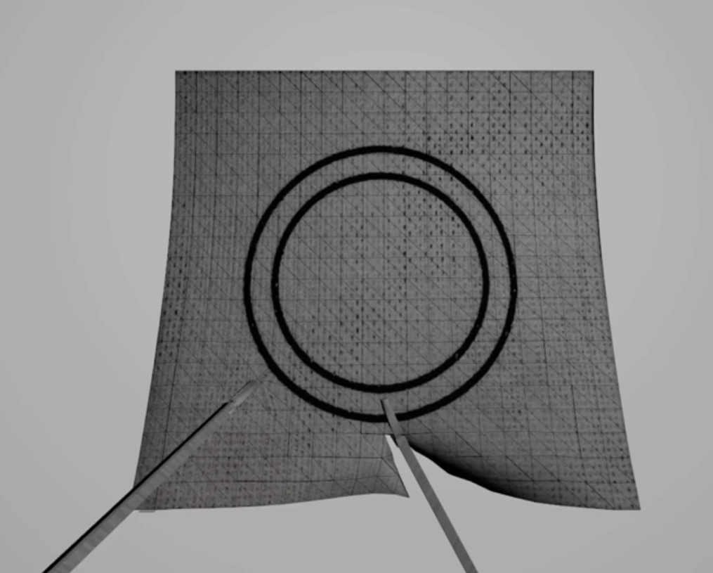
Cloth

Currently iMSTK supports the thin elastic sheets like cloth via PBD formulation which are governed by distance and dihedral constraints. The code below demonstrates the initialization of the PbdModel and its configuration.

auto deformableObj = std::make_shared<PbdObject>("Cloth");
auto pbdModel = std::make_shared<PbdModel>();
pbdModel->setModelGeometry(surfMesh);
pbdModel->configure(/*Number of constraints*/ 2,
                    /*Constraint configuration*/ "Distance 0.1",
                    /*Constraint configuration*/ "Dihedral 0.001",
                    /*Mass*/ 1.0,
                    /*Gravity*/ "0 -9.8 0",
                    /*TimeStep*/ 0.03,
                    /*FixedPoint*/ "1 2 3 4 5 6 7 8 9 10 11",
                    /*NumberOfIterationInConstraintSolver*/ 5);
deformableObj->setDynamicalModel(pbdModel);
deformableObj->setVisualGeometry(surfMesh);
deformableObj->setPhysicsGeometry(surfMesh);

The dihedral constraints require that the mesh supplied is a surface mesh. Note that for the PBD formulation the number of iterations of the solver can determine the eventual stiffness exhibited by the cloth.

Fluids

iMSTK provides two options to simulated fluids: Smoothed-Particle Hydrodynamics (SPH) and PBD. Both of them are particle-based formulations.

Smoothed Particle Hydrodynamics

Smoothed Particle Hydrodynamics (SPH) is one of the widely used methods for simulating fluid flow (and solid mechanics) in distinct areas such as computer graphics, astrophysics, and oceanography among others. SPH is a mesh-free Lagrangian method that employs a kernel function to interpolate fluid properties and spatial derivatives at discrete particle positions.

The SPH model in iMSTK is a form of Weakly Compressible SPH (WSPH) introduced by Becker and Teschner [sph1], but with a number of modifications. In particular, their proposed momentum equation for acceleration update and Tait’s equation for pressure computation was employed. However, two different functions for kernel evaluation and evaluation of kernel derivatives were used, similar to Muller et al. [sph2]. In addition, a variant of XSPH [sph3] is used to model viscosity that is computationally cheaper than the traditional formulation. The forces of surface tension are modeled using a robust formulation proposed by Akinci et al. [sph4] allowing simulation of large surface tension forces in a realistic manner.

During the simulation, each of the SPH particles needs to search for its neighbors within a preset radius of influence of the kernel function (see figure 1). In iMSTK, the nearest neighbor search is achieved using a uniform spatial grid data structure or using spatial hashing based lookup [sph5]. For fluid-solid interaction, the current implementation only supports one-way coupling in which fluid particles are repelled from solids upon collision by penalty force generation.

The code snippet below show creation and configuration of the SPH model and solver.

// Create and configure SPH model
auto sphModel = std::make_shared<SPHModel>();
sphModel->setModelGeometry(fluidGeometry);

auto sphParams = std::make_shared<SPHModelConfig>(particleRadius);
sphParams->m_bNormalizeDensity = true;
sphParams->m_kernelOverParticleRadiusRatio = 6.0;
sphParams->m_viscosityCoeff                = 0.5;
sphParams->m_surfaceTensionStiffness       = 5.0;
sphModel->configure(sphParams);
sphModel->setTimeStepSizeType(TimeSteppingType::realTime);

...

// Configure SPH solver
auto sphSolver = std::make_shared<SPHSolver>();
sphSolver->setSPHObject(fluidObj);
scene->addNonlinearSolver(sphSolver);

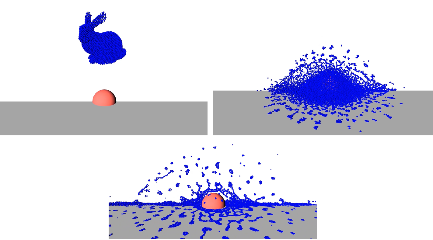
Position based dynamics

Fluids (in this case liquids) are supported in iMSTK via PBD. Constant density constraints are solved within the PBD solution framework in order to achieve the fluid flow. The formulation operates on a set of points.

auto deformableObj = std::make_shared<PbdObject>("Dragon");
deformableObj->setVisualGeometry(fluidMesh);
deformableObj->setCollidingGeometry(fluidMesh);
deformableObj->setPhysicsGeometry(fluidMesh);
auto pbdModel = std::make_shared<PbdModel>();
pbdModel->setModelGeometry(fluidMesh);
pbdModel->configure(/*Number of Constraints*/ 1,
                    /*Constraint configuration*/ "ConstantDensity 1.0 0.3",
                    /*Mass*/ 1.0,
                    /*Gravity*/ "0 -9.8 0",
                    /*TimeStep*/ 0.005,
                    /*FixedPoint*/ "",
                    /*NumberOfIterationInConstraintSolver*/ 2,
                    /*Proximity*/ 0.1,
                    /*Contact stiffness*/ 1.0);
deformableObj->setDynamicalModel(pbdModel);

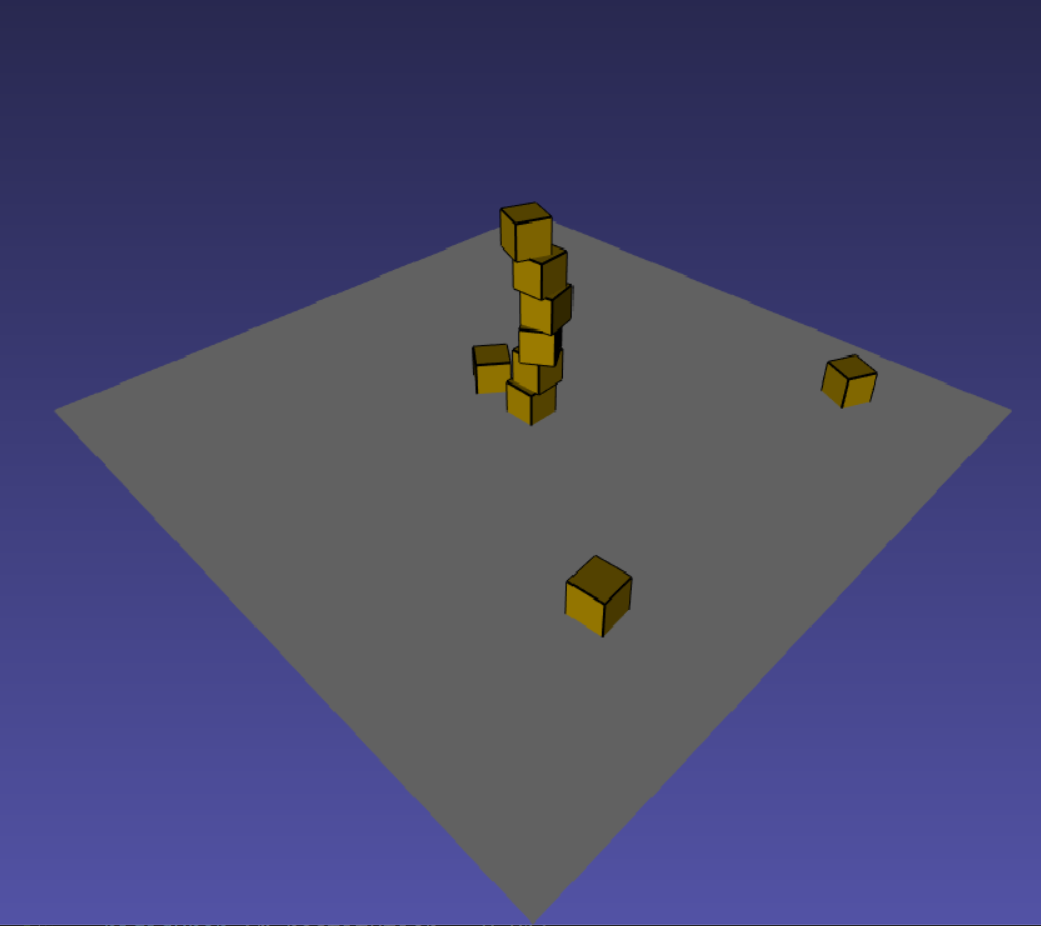
Rigid Body Dynamics

The rigid body dynamics is made available in iMSTK through PhysX. The rigid body can either be static, kinematic or dynamic. Currently cube, sphere, plane and a mesh geometry types can be assigned to the physics geometry of the rigid body dynamics object. Below is the code snippet to configure the rigid body dynamical model and assign it to an object described in 3D by a surface geometry. As can be seen the firction properties of the body can be configured through the RigidBodyPropertyDesc object.

/* create a rigid scene object */
auto rigidObject = std::make_shared<RigidObject>("RigidObject");
rigidObject->setVisualGeometry(cubeGeom);
rigidObject->setCollidingGeometry(cubeGeom);
rigidObject->setPhysicsGeometry(cubeGeom);

/* Create and configure cube dynamic model */
auto rigidModel = std::make_shared<RigidBodyModel>();
auto rigidProp = std::make_shared<RigidBodyPropertyDesc>();
rigidProp->m_dynamicFriction = 0.01;
rigidProp->m_restitution = 0.01;
rigidProp->m_staticFriction = 0.005;

rigidModel->configure(cubeGeom, rigidProp, RigidBodyType::Dynamic);
cubeObj->setDynamicalModel(rigidModel);

Additionally, external force can be added to each dynamic rigid object through RigidBodyModel::addForce() function.

Note

All the rigid bodies in the scene currently interact with every other rigid body in the rigid body world (RigidBodyWorld). This needs to be modified to follow the collision graph of imstk.

Note

For dynamic mesh objects the mesh needs to be convex and can contain a maximum of 256 polygons. These restrictions are placed by the PhysX library due to efficiency considerations.

Computational Algebra

Direct Linear Solvers

iMSTK provides interface to all the direct solvers (based on dense and sparse matrices) that Eigen provide. They are: (a) LU factorization, (b) LDLT, (c) QR factorization, (d) Cholesky factorization.

Iterative Linear Solvers

iMSTK also provides access to Eigen’s iterative solvers like Conjugate Gradient and Gauss Seidel. In addition, the following custom solvers are available:

1. Modified conjugate gradient (MCG): Solves linear system of equations with the symmetric positive definite system matrix along with orthogonal linear projection constraints [mcg].
2. Modified Gauss-Seidel: Similar to modified MCG but solves the linear system by projecting the constraints node-wise at each iteration.
3. PBD solver: Position based dynamics [pbd] formulation generates a list of heterogeneous non-linear set of constraints that need to be solved using nonlinear Gauss-Seidel. PBD solver implements this solution.

External Devices

Most surgical simulators require the users to interact with the software using a hardware interface. For this purpose, iMSTK uses VRPN library [vrpn] to interface with wide number of hardware devices. Currently, iMSTK supports a subset of these devices, specifically, Novint Falcon, Geomagic Touch, OSVR, Arduino, 3D Connexion Navigator and 3D Connexion Space Explorer.

Audio

Simulation of some surgical scenarios require reproduction of the sounds produced during surgery. iMSTK provides the capability to do so via SFML library [sfml]. Features include ability to configure the position of the sound source, position of the listener, attenuation coefficients, sound pitch. Please refer to audio example for details.

Note

Currently, in order to enable the audio capability, iMSTK_AUDIO_ENABLED has to be set to ON at CMake configure time.

Haptic Rendering

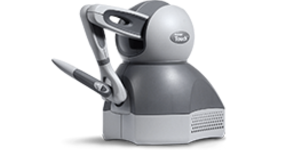
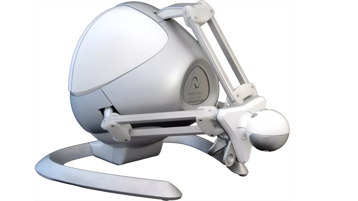
Many medical simulations involve the surgeon feeling the force feedback from the organs through the surgical tools. The ability to allow for algorithms to reproduce this is crucial for the framework. iMSTK currently supports GeoMagic Touch and Novint Falcon devices for force rendering.

GeoMagic Touch

Novint Falcon

An example code on how to instantiate a haptic device is shown below

// Create Device Client
auto client = std::make_shared<HDAPIDeviceClient>(“Phantom1”);

// Create Device Server
auto server = std::make_shared<HDAPIDeviceServer>();
server->addDeviceClient(client);
sdk->addModule(server);

Paralle Support

iMSTK allows CPU based shared memory parallelization using Intel TBB library. imstk::ParallelUtils features utilities that allows users to explot loop-based parallelism.

Below is the sample usage of the paralle for loop in the PointSetToCapsuleCD static function since collision computation can be run independently on each point in the set.

void PointSetToCapsuleCD::computeCollisionData()
{
    m_colData->clearAll();
    ParallelUtils::parallelFor(static_cast<unsigned int>(m_pointSet->getVertexPositions().size()),
        [&](const unsigned int idx)
        {
            const auto& point = m_pointSet->getVertexPosition(idx);
            NarrowPhaseCD::pointToCapsule(point, idx, m_capsule.get(), m_colData);
        });
}

Additional utility functions are available in the same namespace that allow parallel execution of computational kernel over nested indices in 2D and 3D with options to parallelize over a dimension of choice.

Miscellaneous Topics

Object Controllers

The scene objects in the scene can be controlled in real-time by the user through user inputs such as keyboard inputs or movement of the end effector of one of the supported devices. This feature becomes handy for surgical scenarios where the surgical tools are controlled by the user movements.

imstkSceneObject controller class implements this feature. Given a scene object and the device tracker, object control can be instantiated by the following statement

auto controller = std::make_shared<SceneObjectController>(object, trackCtrl);
scene->addObjectController(controller);

At runtime, the scene object’s pose (position and orientation) will be set to that of the device tracker. In addition, imstk provides a utility class for two-jawed laparoscopic tool. Its usage can be found in LaparoscopicToolController example. In addition, a DummyClient class allows for external program to provide the updated pose. This is especially useful when imstk is used as an external library where the main program handles the device control.

Event Handling

Currently, the events are handled in imstk using three different mechanisms which will be unified in the future. Standard key press and mouse events are handled in iMSTK via VTK’s interactor style. Currently pan-zoom-rotate via input from the mouse is achieved through this mechanism. Below is the example of setting a custom callback linked to press of a key

.. // Create a call back on key press of 'b' to take the screen shot"
viewer->setOnCharFunction('b', [&](InteractorStyle\* c) -> bool
{
    screenShotUtility->saveScreenShot();
    return false;
});

Any event triggered by non-standard external devices (eg: foot pedal) is implemented in collision handling or via lambda mechanism of the imstk Module.

File Formats

iMSTK handles a range of file formats for various types of media.

• Surface/Volumetric Meshes: .fbx, .dae, .obj, .stl, .3ds, .ply, .vtk, .vtu
• Texture Formats: .png, .jpg, .bmp, .dds (for Vulkan cubemaps)
• Configuration Files: .config (from vega)
• Misc.: .bou (boundary condition files)

I/O

The file I/O is handled by MeshIO module. Any file format can be loaded using a simple call shown below.

auto objMesh = MeshIO::read(iMSTK_DATA_ROOT"/asianDragon/asianDragon.obj");
auto plyMesh = MeshIO::read(iMSTK_DATA_ROOT"/cube/cube.ply");
auto stlMesh = MeshIO::read(iMSTK_DATA_ROOT"/cube/cube.stl");
auto vtkMesh = MeshIO::read(iMSTK_DATA_ROOT"/cube/cube.vtk");
auto vegaMesh = MeshIO::read(iMSTK_DATA_ROOT"/cube/cube.veg");

Please refer to MeshIOExample for more details on the usage. Currently imstk do not support file output.

Format Check

iMSTK has a set of guidelines for code style formatting and is enfored automatically using uncrustify external library. The check for the code style is embedded on the unit tests. However, in order to make it convenient for the developed, uncrustify_Run project get shipped and build at the time of building iMSTK. Running the executable from the project will modify the code to enforce the code style.

Utilities

Imstk captures commonly used code patterns inside the utilities in order to reduce the amount of code in the application and to quickly create a working application.

API utilities

The namespace imstk::APIUtilities contains utility functions that allows for quick creation and configuring of scene objects.

createVisualAnalyticalSceneObject(imstk::Geometry::Type type,
                                  std::shared_ptr<imstk::Scene> scene,
                                  const std::string objName,
                                  const double scale = 1.,
                                  const imstk::Vec3d t(0.,0.,0.));

Above is a declaration of a utility function that allows creation and do initial transform of any analytical object (that is visual only) in one call. Additional utilities include (a) creation of a colliding scene object that is represented by analytic geometry, (b) an utility to create a nonlinear system, and (c) an utility to print the framerate of the simulation into the standard output window.

More utilities will be added in the future when different usage patterns are identified.

Walk-through Example

This chapter walks through an example scene where a tool controlled by the user through the use of a haptic device interacts with a deformable object (finite element based).

Step 1: Instantiating a simulation manager and setting up the scene

auto sdk = std::make_shared<SimulationManager>();
auto scene = sdk->createNewScene("LiverToolInteraction");
scene->getCamera()->setPosition(0, 2.0, 40.0);

Step 2: Loading model data from a file

auto tetMesh =
imstk::MeshIO::read(iMSTK_DATA_ROOT"/oneTet/oneTet.veg");

if (!tetMesh)
{
    (WARNING) << "Could not read mesh from file.";
    return 1;
}

Step 3: Extracting the surface mesh that is needed for rendering

auto surfMesh = std::make_shared<imstk::SurfaceMesh>();
auto volTetMesh = std::dynamic_pointer_cast<imstk::TetrahedralMesh>(tetMesh);

if (!volTetMesh)
{
    LOG(WARNING) << "Dynamic pointer cast from imstk::Mesh to
    imstk::TetrahedralMesh failed!";

    return 1;
}

volTetMesh->extractSurfaceMesh(surfMesh);

Step 4: Creating a mapping between the volume and surface mesh

auto oneToOneNodalMap = std::make_shared<imstk::OneToOneMap>();
oneToOneNodalMap->setMaster(tetMesh);
oneToOneNodalMap->setSlave(surfMesh);
oneToOneNodalMap->compute();

Step 5: Setting up the dynamic model that will be used in the scene

auto dynaModel = std::make_shared<FEMDeformableBodyModel>();
dynaModel->configure(iMSTK_DATA_ROOT"/oneTet/oneTet.config");
dynaModel->initialize(volTetMesh);

// Create and add Backward Euler time integrator
auto timeIntegrator = std::make_shared<BackwardEuler>(0.001);

dynaModel->setTimeIntegrator(timeIntegrator);

Step 6: Creating a deformable object and adding it to the scene

auto deformableObj = std::make_shared<DeformableObject>("Dragon");
deformableObj->setVisualGeometry(surfMesh);
deformableObj->setPhysicsGeometry(volTetMesh);
deformableObj->setPhysicsToVisualMap(oneToOneNodalMap); //assign the computed map
deformableObj->setDynamicalModel(dynaModel);
deformableObj->initialize();
scene->addSceneObject(deformableObj);

Step 7: Creating a nonlinear system

auto nlSystem = std::make_shared<NonLinearSystem>(dynaModel->getFunction(),
                                                   dynaModel->getFunctionGradient());

std::vector<LinearProjectionConstraint> projList;

for (auto i : dynaModel->getFixNodeIds())
{
    auto s = LinearProjectionConstraint(i, false);
    s.setProjectorToDirichlet(i);
    s.setValue(Vec3d(0.001, 0, 0));
    projList.push_back(s);
}

nlSystem->setLinearProjectors(projList);
nlSystem->setUnknownVector(dynaModel->getUnknownVec());
nlSystem->setUpdateFunction(dynaModel->getUpdateFunction());
nlSystem->setUpdatePreviousStatesFunction(dynaModel->getUpdatePrevStateFunction());

Step 8: Creating a linear solver and adding it to the nonlinear system

// create a linear solver
auto cgLinSolver = std::make\shared<ConjugateGradient>();

// create a non-linear solver and add to the scene
auto nlSolver = std::make\shared<NewtonSolver>();

nlSolver->setLinearSolver(cgLinSolver);
nlSolver->setSystem(nlSystem);
//nlSolver->setToFullyImplicit();
scene->addNonlinearSolver(nlSolver);

Step 9: Setting up the haptics interface

// Device clients
auto client = std::make_shared<imstk::HDAPIDeviceClient>("Default Device");

// Device Server
auto server = std::make_shared<imstk::HDAPIDeviceServer>();

server->addDeviceClient(client);

sdk->addModule(server);

Step 10: Creating tool-related scene objects and adding them to the scene

// Load tool mesh from a file
auto pivot = apiutils::createAndAddVisualSceneObject(scene,
                                                     iMSTK_DATA_ROOT"/laptool/pivot.obj",
                                                     "pivot");

// Or analytical object
auto sphere0Obj = apiutils::createCollidingAnalyticalSceneObject(imstk::Geometry::Type::Sphere,
                                                                 scene,
                                                                 "Sphere0",
                                                                 3,
                                                                 Vec3d(1, 0.5, 0));
auto trackingCtrl = std::make_shared<imstk::DeviceTracker>(client);

auto lapToolController = std::make_shared<imstk::SceneObjectController>(sphere0Obj,
                                                                        trackingCtrl);

scene->addObjectController(lapToolController);

Step 11: Creating the collision interaction graph

scene->getCollisionGraph()->addInteractionPair(deformableObj,
                                               sphere0Obj,
                                               CollisionDetection::Type::MeshToSphere,
                                               CollisionHandling::Type::Penalty,
                                               CollisionHandling::Type::None);

Step 12: Setting up camera parameters in the scene (if necessary)

// Set Camera configuration
auto cam = scene->getCamera();

cam->setPosition(imstk::Vec3d(0, 20, 20));
cam->setFocalPoint(imstk::Vec3d(0, 0, 0));

Step 13: Running the simulation

sdk->setCurrentScene(scene);
sdk->startSimulation(true);

Bibliography

[mcg]

Uri M. Ascher and Eddy Boxerman. 2003. On the modified conjugate gradient method in cloth simulation. Vis. Comput. 19, 7-8 (December 2003), 526-531.

[pbd]

Matthias Müller, Bruno Heidelberger, Marcus Hennix, and John Ratcliff. 2007. Position based dynamics. J. Vis. Comun. Image Represent. 18, 2 (April 2007), 109-118.

[vrpn]

Russell M. Taylor, II, Thomas C. Hudson, Adam Seeger, Hans Weber, Jeffrey Juliano, and Aron T. Helser. 2001. VRPN: a device-independent, network-transparent VR peripheral system. In Proceedings of the ACM symposium on Virtual reality software and technology (VRST ‘01). ACM, New York, NY, USA, 55-61.

[sfml]

Simple and Fast Multimedia Library: https://github.com/SFML/SFML

[sph1]

Markus Becker and Matthias Teschner, “Weakly compressible SPH for free surface flows”. In Proceedings of the ACM SIGGRAPH/Eurographics symposium on Computer Animation, 209-217 (2007).

[sph2]

Matthias Müller, David Charypar, and Markus Gross, “Particle-based fluid simulation for interactive applications”. In Proceedings of the 2003 ACM SIGGRAPH/Eurographics symposium on Computer Animation, 154-159 (2003).

[sph3]

Hagit Schechter and Robert Bridson, “Ghost SPH for animating water”. ACM Transaction on Graphics, 31, 4, Article 61 (July 2012).

[sph4]

Nadir Akinci, Gizem Akinci, and Matthias Teschner, “Versatile surface tension and adhesion for SPH fluids”. ACM Transaction on Graphics, 32, 6, Article 182 (November 2013).

[sph5]

Teschner, M., Heidelberger, B., Müller, M., Pomeranets, D., and Gross, M, “Optimized spatial hashing for collision detection of deformable objects”. Proc. VMV, 47–54.

[cd1]

Christer Ericson. Real-Time Collision Detection. CRC Press, Inc., Boca Raton, FL, USA, 2004.